MBHB’s Fisher matrix with WeJAX

here we provide some examples of Fisher matrix computation for Massive Black Hole Binary (MBHB) systems using wejax.

There are currently no jax based MBHB waveform generators. Therefore, in this tutorial, we will only use the “finite differeces” (findiff) jacobian computation provided by wejax

Libraries

all libraries are pip installable.

If you are setting up the development environment using poetry you can install them using the lisabeta group.

poetry install --with lisabeta

import time
import numpy as np
import matplotlib.pyplot as plt
import jax
import jax.numpy as jnp
from wejax.jacobian import findiff
from wejax.fim import matched_filter_gaussian_fim as fim
from wejax.errors import correlation_matrix, plot_correlation_matrix, stddevs
import lisabeta.lisa.lisa as lisa
from lisaconstants import (
    SIDEREALYEAR_J2000DAY as DAYS_IN_A_YEAR,
    ASTRONOMICAL_UNIT as AU_SI,
)
from fomweb.analytic_noise import get_noise_aet

Note that we need to enable the 64bit support of jax.

jax.config.update("jax_enable_x64", True)

MBHB template

here we define a class that provides the MBHB template meethod tdi (i.e. the waveform generator). This is a simple implementation based on the lisabeta MBHB fast waveform generator.

Note that the choice of the physical parameters taken as inputs by the template method defines the variable wrt which we will differentiate the likelihood and, eventually, the errors that we will compute.

Here we will take the $log_{10}$ of the masses and of distance, thus the corresponding errors will be relative errors.

class MBHBTempl:
    """
    MBHB template class/

    :param dict wf_params: waveform parameters.
    :param array fgrid: frequency grid (list or array).
    """

    #:list: template parameters
    mbhb_pars = [
        "m1_log10",
        "m2_log10",
        "chi1",
        "chi2",
        "dist_log10",
        "inc_cos",
        "beta_sin",
        "lambda",
        "Deltat",
        "psi",
        "phi",
    ]

    def __init__(self, wf_params, fgrid):

        #:dict: waveform parameters.
        self.wfp = wf_params
        self.fgrid = np.array(fgrid)

    def to_tpl(self, pars):
        """
        Transforms a list of template parameters (in the form defined by
        `MBHBTempl.mbhb_pars`) into a template parameters dictionnary
        of the form required by lisabeta fast MBHB generator.

        :param tuple pars: template parameters.

        :return: lisabeta template parameters dictionnary
        :rtype: dict
        """
        _tpl = {_key: pars[_ind] for _ind, _key in enumerate(self.mbhb_pars)}
        for _key in ["m1", "m2", "dist"]:
            _tpl[_key] = 10 ** _tpl[f"{_key}_log10"]
        _tpl["beta"] = jnp.arcsin(_tpl["beta_sin"])
        _tpl["inc"] = jnp.arccos(_tpl["inc_cos"])
        return _tpl

    def to_pars(self, tpl):
        """
        Transforms a lisabeta template parameters dictionnary into a
        list of template parameters (in the form defined by `MBHBTempl.mbhb_pars`).

        :param dict tpl: lisabeta template parameters dictionnary

        :return: list of template parameters
        :rtype: list
        """
        _tpl = tpl.copy()
        for _key in ["m1", "m2", "dist"]:
            _tpl[f"{_key}_log10"] = jnp.log10(tpl[_key])
        _tpl["beta_sin"] = np.sin(_tpl["beta"])
        _tpl["inc_cos"] = np.cos(_tpl["inc"])
        return [_tpl[_key] for _key in self.mbhb_pars]

    def tdi_fs(self, pars):
        """
        Generate the template frequency serie for the 3 channels
        (A, E, T) on the template frequency frequency grid.

        :param tuple pars: template parameters.

        :return: the frequency series as a dictionnary bearing
                 - the frequency grid
                 - the series of all channels and modes
        :rtype: dict
        """
        # Here we generate the WF on the inner defined freq grid.
        # _tdi is a dictionnary bearing for all modes:
        #     - frequencies
        #     - overall phase
        #     - real and imaginary parts of the amplitudes of each channel.
        _tdi = lisa.GetCAmpPhaseTDI(
            lisa.GenerateLISATDI_SMBH(self.to_tpl(pars), **self.wfp)
        )

        # Here we interpolate and compose phases and amplitudes
        # to obtain the signal on self.fgrid
        return lisa.EvaluateTDIFreqseries(_tdi, self.fgrid)

    def tdi(self, *pars):
        """
        Generates the MBHB waveform given a set of parameters.

        :param float par: the template parameters as defined by `MBHBTempl.mbhb_pars`

        :return: a Nf x Nc jax array with the A and E signals (we ignore the T channel)
        :rtype: jax.ndarray
        """
        _tdi = self.tdi_fs(pars)

        return jnp.sum(
            jnp.array(
                [
                    [_tdi[_md][f"chan{_ind + 1}"] for _ind in range(2)]
                    for _md in _tdi["modes"]
                ],
            ),
            axis=0,
        ).T

Test waveform generation

let’s first test the template class defined above.

We consider circular orbits with fixed arm:

ORBITS = {
    "OrbitOmega": 2 * jnp.pi / DAYS_IN_A_YEAR / 24 / 3600,  # Orbiting with Eart (Omega)
    "OrbitPhi0": 0,
    "Orbitt0": 0,
    "OrbitR": AU_SI,  # Orbiting with Eart (Radius)
    "OrbitL": 2500000000.0,  # Costellation Arm
}

We consider a waveform in the $[2\cdot10^{-5}, 0.1] Hz$. We use tdi 2 and the IPRPhenomD approximant (thus we will only have the $(2,2)$ mode generated.

WF_PARS = {
    "minf": 2e-5,
    "maxf": 0.1,
    "fend": None,
    "tmin": None,
    "tmax": None,
    "phiref": 0.0,
    "fref_for_phiref": 0.0,
    "toffset": 0.0,
    "TDI": "TDI2AET",
    "acc": 1e-4,
    "order_fresnel_stencil": 0,
    "approximant": "IMRPhenomD",
    "responseapprox": "full",
    "frozenLISA": False,
    "TDIrescaled": True,
    "LISAconst": ORBITS,
}

We define a logarithmic 10000 points frequency grid on the waveform frequency range.

FGRID = np.logspace(-5 + np.log10(2), -1, 10000)

And finally we define the following test MBHB system

SRC_PARS = {
    "m1": 47258.329389317725,
    "m2": 17741.67061068228,
    "chi1": 0.0,
    "chi2": 0.0,
    "Deltat": 0.5,
    "dist": 143838.55484688256,
    "inc": 1.125884012332375,
    "phi": 0.3067042906681201,
    "lambda": 0.6456813346495229,
    "beta": 0.08988736148757666,
    "psi": 1.330950805261161,
}

Now let’s instantiate the template

mbhb_tpl = MBHBTempl(WF_PARS, FGRID)

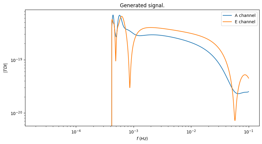
And generate the tdi signal

mbhb_tdi = mbhb_tpl.tdi(*mbhb_tpl.to_pars(SRC_PARS))

_, _ax = plt.subplots(1, 1, figsize=(10, 5))
_ax.plot(FGRID, jnp.abs(mbhb_tdi[:, 0]), label="A channel")
_ax.plot(FGRID, jnp.abs(mbhb_tdi[:, 1]), label="E channel")

_ax.set_title("Generated signal.")
_ax.set_xlabel("$f~(Hz)$")
_ax.set_ylabel("$|TDI|$")
_ax.set_xscale("log")
_ax.set_yscale("log")

_ = _ax.legend()

Let’s also have a look at the execution time of the wf generator

_pars = mbhb_tpl.to_pars(SRC_PARS)
%timeit mbhb_tpl.tdi(*_pars)

3.03 ms ± 141 μs per loop (mean ± std. dev. of 7 runs, 100 loops each)

Differentiation

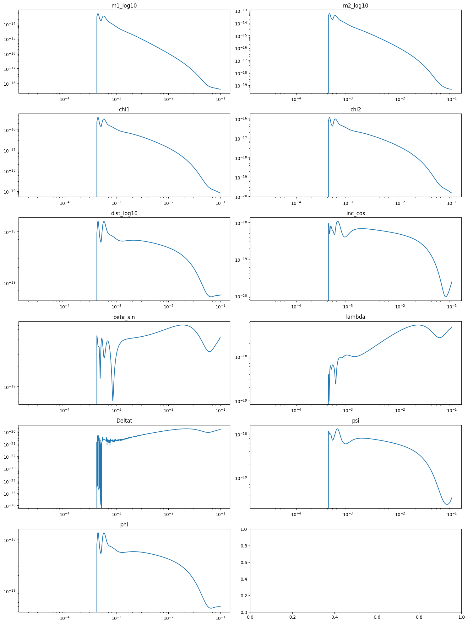
Let’s now use the wejax function for finite differencies differentiation findiff to compute the gradient of the signal generated by the template.

First of all we define the finite different steps for all the parameters.

# "m1", "m2", "chi1", "chi2", "dist_log10", "inc_cos", "beta_sin", "lambda", "Deltat", "psi", "phi"

STEPS = [1e-05, 1e-05, 1e-06, 1e-06, 1e-06, 1e-06, 1e-05, 1e-05, 1e-09, 1e-06, 1e-05]

Instantiate the gardient function

mbhb_grad_gen = findiff(mbhb_tpl.tdi, argnums=list(range(11)), steps=STEPS)

And compute the gradient for the test system defined above

mbhb_grad = mbhb_grad_gen(*_pars)

_fig, _axs = plt.subplots(6, 2, figsize=(15, 20))
for _ind in range(11):
    _ax = _axs[_ind // 2][_ind % 2]
    _ax.plot(FGRID, np.abs(mbhb_grad[:, 0, _ind]))
    _ax.set_xscale("log")
    _ax.set_yscale("log")
    _ax.set_title(mbhb_tpl.mbhb_pars[_ind])

_fig.tight_layout()

Let’s have a quick look at the timing.

%timeit mbhb_grad_gen(*_pars)

95.8 ms ± 3.14 ms per loop (mean ± std. dev. of 7 runs, 10 loops each)

Computing Fisher Matrix and errors

here we proceed with the compiutation of the fisher matrix and of the corresponding errors.

Defining the noise

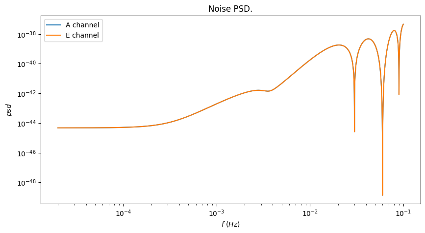
first of all we need to define the noise. For this we use a the analytical scird noise model from the get_noise_aet function of the fomweb package. We consider the confusion noise fro 1 year of observation.

First we generate the psd

noise_psd = get_noise_aet(FGRID, model="scird", duration=1.0)

_, _ax = plt.subplots(1, 1, figsize=(10, 5))
_ax.plot(FGRID, noise_psd[:, 1], label="A channel")
_ax.plot(FGRID, noise_psd[:, 2], label="E channel")
_ax.set_title("Noise PSD.")
_ax.set_xlabel("$f~(Hz)$")
_ax.set_ylabel("$psd$")
_ax.set_xscale("log")
_ax.set_yscale("log")


_ = _ax.legend()

Then we compute the corresponding list of 2 x 2 inverse noise covariance matrices (one per frequency).

inv_noise_cov = np.array([np.diag(1 / _item[1:3]) for _item in noise_psd])

FIM computation

Let’s instanciate the FIM generator for the already instanciated MBHB gradient generator and for the defined inverse noise covariance.

Note that since we are working on a non equal grid we should set the df parameter to one and pass to the sum_func parameter a wrapped version of np.trapezoid that works on the desired frequency grid.

mbhb_fim_gen = fim(
    jacobian=mbhb_grad_gen,
    noise_cov=inv_noise_cov,
    df=1.0,
    should_invert_noise_cov=False,
    sum_func=lambda vals, dx, axis: np.trapezoid(vals, x=FGRID, axis=-1),
)

Then let’s compute the fim for the test system.

mbhb_fim = mbhb_fim_gen(*_pars)

Here is the plot of the corresponding covariance matrix.

_, _ax = plt.subplots(1, 1, figsize=(12, 7))
_ = plot_correlation_matrix(
    correlation_matrix(fim=mbhb_fim), param_names=mbhb_tpl.mbhb_pars, ax=_ax
)

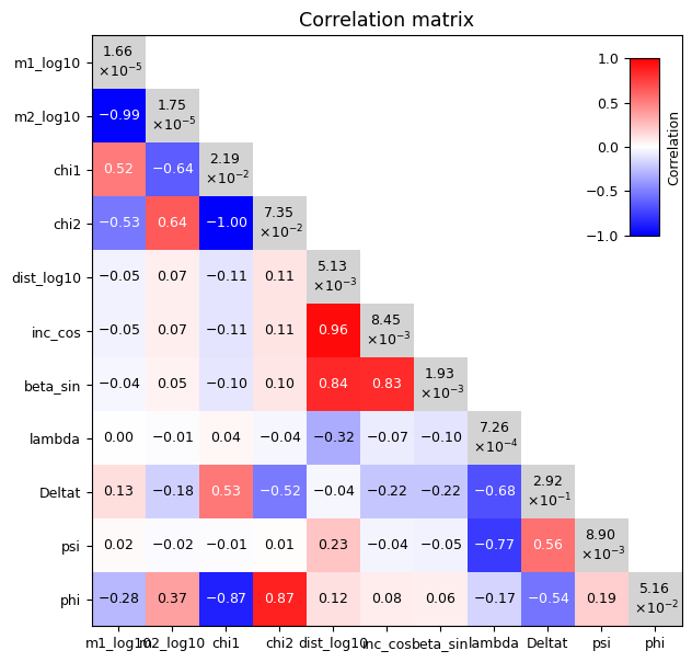
And here are the computed errors

{
    mbhb_tpl.mbhb_pars[_ind]: float(_val)
    for _ind, _val in enumerate(stddevs(fim=mbhb_fim))
}

{'m1_log10': 1.656996345102525e-05,
 'm2_log10': 1.745047430212579e-05,
 'chi1': 0.021906617330913272,
 'chi2': 0.07354942156473049,
 'dist_log10': 0.00512824908806289,
 'inc_cos': 0.008448297934872675,
 'beta_sin': 0.0019330166455207853,
 'lambda': 0.0007263065428983844,
 'Deltat': 0.29188863033183665,
 'psi': 0.008895699194008866,
 'phi': 0.05160223364025217}

Now let’s have a look at the timing.

%timeit mbhb_fim_gen(*_pars)

196 ms ± 5.25 ms per loop (mean ± std. dev. of 7 runs, 10 loops each)

Computing a set of FIM

now let’s try a more real case scenario. We build NSAMPLES systems by randomizing the angles of the test system. Then we compute the fim for each one of these systems.

mbhb_tpl = MBHBTempl(WF_PARS, FGRID)
mbhb_grad_gen = findiff(mbhb_tpl.tdi, argnums=list(range(11)), steps=STEPS)
mbhb_fim_gen = fim(
    jacobian=mbhb_grad_gen,
    noise_cov=inv_noise_cov,
    df=1.0,
    should_invert_noise_cov=False,
    sum_func=lambda vals, dx, axis: np.trapezoid(vals, x=FGRID, axis=-1),
)

NSAMPLES = 100


def draw_random(tpl):
    _rand = tpl.copy()
    _rand["phi"] = np.random.uniform(low=-np.pi, high=np.pi)
    _rand["inc"] = np.arccos(np.random.uniform(low=-1.0, high=1.0))
    _rand["lambda"] = np.random.uniform(low=-np.pi, high=np.pi)
    _rand["beta"] = np.arcsin(np.random.uniform(low=-1.0, high=1.0))
    _rand["psi"] = np.random.uniform(low=0.0, high=np.pi)

    return mbhb_tpl.to_pars(_rand)


mbhb_rnd = np.array([draw_random(SRC_PARS) for _ in range(NSAMPLES)])

_etime = time.time()
fims = [mbhb_fim_gen(*_pars) for _pars in mbhb_rnd]
print(time.time() - _etime)

19.361433267593384

Note that since lisabeta is not jax friendly we cannot exploit jax vectorization. For example the command below would fail because of an illegal casting.