Estimation errors
This module provides functions to compute and plot error covariance and correlation matrices.
Error covariance matrix
The errors on the estimated parameters can be characterized by their covariance matrix \(\Sigma\), which is defined as the inverse of the Fisher information matrix,
The diagonal elements of \(\Sigma\) provide the variances of the estimated parameters, and the off-diagonal elements describe the correlations.
- wejax.errors.covariance_matrix(fim, *, argnums=None, rtol=None)[source]
Compute the error covariance matrix from the Fisher information matrix.
If the matrix is singular, use
argnumsto select the parameters for which the error covariance matrix is computed. Ifrtolis notNone, the Moore-Penrose pseudo-inverse is computed.Examples
>>> cov = covariance_matrix(fim)
Fixing some parameters yields a different covariance matrix:
>>> cov2 = covariance_matrix(fim, argnums=(0, 1))
>>> np.testing.assert_array_almost_equal(cov2, cov[..., :2, :2])
False
- Parameters:
F (Array-like of shape
(..., Np, Np)) – Fisher information matrix. Here,Npis the number of parameters.argnums (
Sequence[int] |None, default:None) – Indices of the parameters for which the error covariance matrix is computed. By default, the error covariance matrix is computed for all parameters.rtol (
float|None, default:None) –Cutoff parameter for small singular values.
Singular values smaller than
rtoltimes the largest singular value are considered zero and the function returns the Moore-Penrose pseudo-inverse. IfNone, the exact inverse is computed.
- Returns:
Error covariance matrix. Here,
Nais the number of parameters for which the error covariance matrix is computed (length ofargnums).- Return type:
Array
- wejax.errors.stddevs(*, fim=None, cov=None)[source]
Compute parameter standard deviations.
You can provide the noise covariance matrix as input, to avoid inverting the Fisher information matrix.
Examples
>>> a = stddevs(fim=fim)
>>> cov = covariance_matrix(fim)
>>> b = stddevs(cov=cov)
>>> np.testing.assert_array_almost_equal(a, b)
True
- Parameters:
fim (
Array|ndarray|bool|number|bool|int|float|complex|TypedNdArray|None, default:None) – Fisher information matrix. Here,Npis the number of parameters.cov (
Array|ndarray|bool|number|bool|int|float|complex|TypedNdArray|None, default:None) – Error covariance matrix. Here,Npis the number of parameters.
- Returns:
Standard deviations.
- Return type:
Array
Correlation matrix
The correlation matrix \(P\) is defined as the normalized covariance matrix, i.e., the matrix of the standard deviations and the correlation coefficients.
- wejax.errors.correlation_matrix(*, fim=None, cov=None)[source]
Compute the correlation matrix (normalized covariance matrix).
You can provide the noise covariance matrix as input, to avoid inverting the Fisher information matrix.
Examples
>>> a = correlation_matrix(fim=fim)
>>> cov = covariance_matrix(fim)
>>> b = correlation_matrix(cov=cov)
>>> np.testing.assert_array_almost_equal(a, b)
True
- Parameters:
fim (
Array|ndarray|bool|number|bool|int|float|complex|TypedNdArray|None, default:None) – Fisher information matrix. Here,Npis the number of parameters.cov (
Array|ndarray|bool|number|bool|int|float|complex|TypedNdArray|None, default:None) – Error covariance matrix. Here,Npis the number of parameters.
- Returns:
Correlation matrix.
- Return type:
Array
Plotting
You can plot the error covariance matrix using the function
wejax.errors.plot_covariance_matrix().
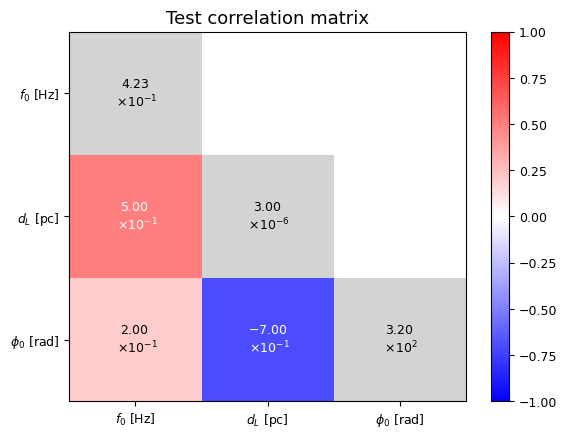
- wejax.errors.plot_correlation_matrix(corr, *, ax=None, param_names=None, param_units=None, title='Correlation matrix', cmap='bwr', show_cbar=True, font_size=9, label_rotation=0)[source]
Plot the correlation matrix.
Examples
>>> corr = correlation_matrix(fim=fim)
>>> names = ["$f_0$", "$d_L$", "$\phi_0$"]
>>> units = ["Hz", "Mpc", "rad"]
>>> fig, ax = plot_correlation_matrix(corr, param_names=names, param_units=units)
>>> fig.savefig("correlation_matrix.pdf", bbox_inches="tight")
- Parameters:
corr (
Array|ndarray|bool|number|bool|int|float|complex|TypedNdArray) – Correlation matrix. Here,Npis the number of parameters.ax (
Axes|None, default:None) – Matplotlib axes. If None, a new figure is created.param_names (
Sequence[str] |None, default:None) – Parameter names. By default, the parameters are labeled with their indices.param_units (
Sequence[str] |None, default:None) – Parameter units. By default, the parameters are labeled without units.title (
str, default:'Correlation matrix') – Figure title.cmap (
str, default:'bwr') – Colormap. See matplotlib colormaps.show_cbar (
bool, default:True) – If True, show colorbar.font_size (
float, default:9) – Font size.label_rotation (
float, default:0) – Rotation angle for x-axis parameter labels.
- Return type:
tuple[Figure,Axes]- Returns:
Figure – Matplotlib figure.
Axes – Matplotlib axes.