GBs’ Fisher matrix with WeJAX
In this notebook, we’ll see how to compute Fisher Information Matrices (FIM) for galactic binary systems using wejax.
We rely on a jax implementation of the GB fast waveform fastgb which is available from pypi pip install fastgb.
Setup
poetry install --with fastgb
import time
import numpy as np
import matplotlib.pyplot as plt
import jax
import jax.numpy as jnp
from wejax.jacobian import autograd
from wejax.fim import matched_filter_gaussian_fim as fim
from wejax.errors import correlation_matrix, plot_correlation_matrix, stddevs
from fastgb import fastgb
from lisaorbits import EqualArmlengthOrbits
from fomweb.analytic_noise import get_noise_aet
/builds/lisamission/wejax/.venv/lib/python3.12/site-packages/tqdm/auto.py:21: TqdmWarning: IProgress not found. Please update jupyter and ipywidgets. See https://ipywidgets.readthedocs.io/en/stable/user_install.html
  from .autonotebook import tqdm as notebook_tqdm
jax.config.update("jax_enable_x64", True) # enable the 64bit support of `jax`.
GB template
We encapsulate the fast waveform template in a class which is the interface to the fastgb waveform provider.
As for MBHB, the choice of the physical parameters taken as inputs by the template method defines the variable wrt which we will differentiate the likelihood and, eventually, the errors that we will compute.
Here we will take the $log_{10}$ of the amplitude and frequency derivative, thus the corresponding errors will be relative errors. We will also consider the cosinus of the inclination angle and sinus of the eclicptic latitude. The central frequency is given in mHz.
class GBTempl:
    """
    GB template class

    :param dict wf_params: waveform parameters.
    """

    #:list: template parameters
    gb_pars = [
        "freq_mHz",
        "fdot_log10",
        "ampl_log10",
        "beta_sin",
        "lambda",
        "psi",
        "incl_cos",
        "phi0",
    ]

    def __init__(
        self, wf_params, T=365 * 24 * 3600, dt=5, N=128, noise_model="SciRDv1"
    ):

        #:dict: waveform parameters.
        self.wfp = wf_params

        #:class: fast waveform generator.
        self.wfm = fastgb.FastGB(delta_t=dt, T=T, N=N, orbits=EqualArmlengthOrbits())

        # frequency grid
        X, _, _, kmin = self.wfm.get_fd_tdixyz(jnp.array(wf_params).reshape(-1, 8))
        self.df = 1 / self.wfm.T
        self.kmin = kmin[0]
        self.fgrid = self.df * np.arange(self.kmin, self.kmin + X.shape[1])

    def to_tpl(self, pars):
        """
        Transforms a list of template parameters (in the form defined by
        `GBTempl.gb_pars`) into a template parameters as required by fastgb.

        :param tuple pars: template parameters.

        :return: template parameters
        :rtype: array
        """
        nf0, log_fdot, log_ampl, sinbet, lamb, psi, cosin, phi0 = pars
        ampl = 10**log_ampl
        fdot = 10**log_fdot
        incl = jnp.arccos(cosin)
        beta = jnp.arcsin(sinbet)
        f0 = nf0 * 1e-3
        return jnp.array([f0, fdot, ampl, beta, lamb, psi, incl, phi0])

    def to_pars(self, tpl):
        """
        Transforms a fastgb into template parameterization. (in the form defined by `GBTempl.gb_pars`).

        :param list tpl: fastgb parameter list

        :return: list of template parameters
        :rtype: list
        """
        _tpl = tpl.copy()
        _tpl[1] = np.log10(_tpl[1])
        _tpl[2] = np.log10(_tpl[2])
        _tpl[6] = np.cos(_tpl[6])
        _tpl[3] = np.sin(_tpl[3])
        _tpl[0] = _tpl[0] * 1e3
        return _tpl

    def tdi(self, *pars):
        """
        Generate the template frequency serie for the TDI channels
        (A, E).

        :param tuple pars: template parameters.

        :return: a Nf x Nc jax array with the A and E signals (we ignore the T channel)
        :rtype: jax.ndarray
        """
        X, Y, Z, _ = self.wfm.get_fd_tdixyz(self.to_tpl(pars).reshape(-1, 8))
        A, E, _ = (
            jnp.array((Z[0] - X[0]) / jnp.sqrt(2.0)),
            jnp.array((X[0] - 2.0 * Y[0] + Z[0]) / jnp.sqrt(6.0)),
            jnp.array((X[0] + Y[0] + Z[0]) / jnp.sqrt(3.0)),
        )
        return jnp.stack([A, E], axis=1)
Test waveform generation
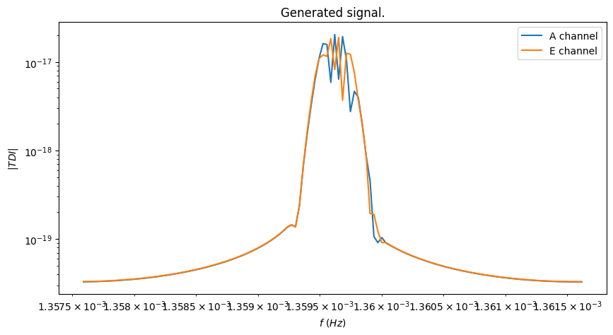
Let’s first test the template class defined above for the following binary system:
SRC_PARS = np.array(
    [
        0.00135962,  # f0 Hz
        8.94581279e-19,  # fdot "Hz^2
        1.07345e-22,  # ampl strain
        0.312414,  # eclipticlatitude radian
        -2.75291,  # eclipticLongitude radian
        3.5621656,  # polarization radian
        0.523599,  # inclination radian
        3.0581565,  # initial phase radian
    ]
)
gb_tpl = GBTempl(SRC_PARS)
gb_tdi = gb_tpl.tdi(*gb_tpl.to_pars(SRC_PARS))
_, _ax = plt.subplots(1, 1, figsize=(10, 5))
_ax.plot(gb_tpl.fgrid, jnp.abs(gb_tdi[:, 0]), label="A channel")
_ax.plot(gb_tpl.fgrid, jnp.abs(gb_tdi[:, 1]), label="E channel")

_ax.set_title("Generated signal.")
_ax.set_xlabel("$f~(Hz)$")
_ax.set_ylabel("$|TDI|$")
_ax.set_xscale("log")
_ax.set_yscale("log")

_ = _ax.legend()
Let’s also have a look at the execution time of the wf generator
_pars = gb_tpl.to_pars(SRC_PARS)
%timeit gb_tpl.tdi(*_pars)
33 ms ± 823 μs per loop (mean ± std. dev. of 7 runs, 10 loops each)
Auto differentiation with JAX
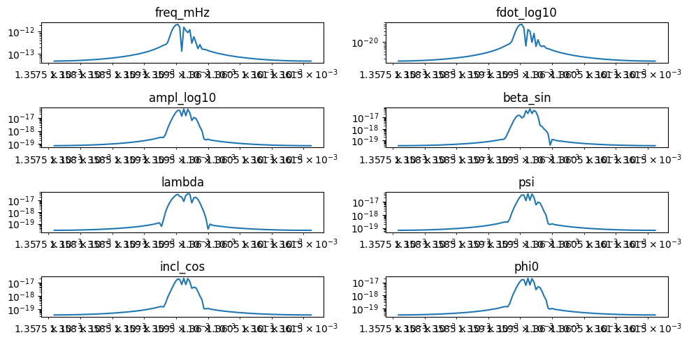
Let’s now use the wejax function for auto differentiation autograd to compute the Jacobian of the signal generated by the template.
gb_grad_gen = autograd(gb_tpl.tdi, argnums=list(range(8)))
gb_grad = gb_grad_gen(*_pars)
_fig, _axs = plt.subplots(4, 2, figsize=(10, 5))
for _ind in range(8):
    _ax = _axs[_ind // 2][_ind % 2]
    _ax.plot(gb_tpl.fgrid, np.abs(gb_grad[:, 0, _ind]))
    _ax.set_xscale("log")
    _ax.set_yscale("log")
    _ax.set_title(gb_tpl.gb_pars[_ind])
_fig.tight_layout()
and corresponding timing
%timeit gb_grad_gen(*_pars)
196 ms ± 3.62 ms per loop (mean ± std. dev. of 7 runs, 10 loops each)
Computing Fisher Matrix and errors
Defining the noise
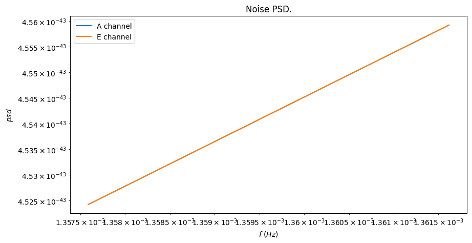
We use the analytical scird noise model from the fomweb package. We consider the confusion noise from 1 year of observation.
We compute its inverse once for all, to speed up the wejax FIM computation.
noise_psd = get_noise_aet(gb_tpl.fgrid, model="scird", duration=1.0)
inv_noise_cov = np.array([np.diag(1 / _item[1:3]) for _item in noise_psd])
_, _ax = plt.subplots(1, 1, figsize=(10, 5))
_ax.plot(gb_tpl.fgrid, noise_psd[:, 1], label="A channel")
_ax.plot(gb_tpl.fgrid, noise_psd[:, 2], label="E channel")
_ax.set_title("Noise PSD.")
_ax.set_xlabel("$f~(Hz)$")
_ax.set_ylabel("$psd$")
_ax.set_xscale("log")
_ax.set_yscale("log")
_ = _ax.legend()
FIM computation
Let’s instanciate the FIM generator for the already instanciated GB gradient generator and for the defined inverse noise covariance.
gb_fim_gen = fim(
    jacobian=gb_grad_gen,
    noise_cov=inv_noise_cov,
    df=gb_tpl.df,
    should_invert_noise_cov=False,
)
gb_fim = gb_fim_gen(*_pars)
_, _ax = plt.subplots(1, 1, figsize=(12, 7))
_ = plot_correlation_matrix(
    correlation_matrix(fim=gb_fim), param_names=gb_tpl.gb_pars, ax=_ax
)
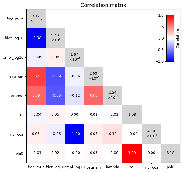
As expected see correlation between
f0 and fdot,
amplitude and inclination,
initial phase and polarisation
and sky location
Let’s have a look at the timing again
%timeit gb_fim_gen(*_pars)
219 ms ± 4.4 ms per loop (mean ± std. dev. of 7 runs, 1 loop each)
The associated errors lower bound read
{gb_tpl.gb_pars[_ind]: float(_val) for _ind, _val in enumerate(stddevs(fim=gb_fim))}
{'freq_mHz': 3.1731512541085714e-06,
 'fdot_log10': 95.83621590863899,
 'ampl_log10': 0.1874918455568794,
 'beta_sin': 0.026931189199108946,
 'lambda': 0.02541189601441582,
 'psi': 1.5905747769242788,
 'incl_cos': 0.400228016627111,
 'phi0': 3.1818812523267956}
Computing a set of FIM
We’ll see the potential of the JAX acceleration by computing a large number of FIM for a given list of systems.
We’ll simply randomize over the angles on the example system given here.
NSAMPLES = 100
gb_rnd = np.tile(SRC_PARS.reshape(8, -1), NSAMPLES)

gb_pars = [
    "freq_mHz",
    "fdot_log10",
    "ampl_log10",
    "beta_sin",
    "lambda",
    "psi",
    "incl_cos",
    "phi0",
]

gb_rnd[gb_tpl.gb_pars.index("phi0"), :] = np.random.uniform(low=-np.pi, high=np.pi)
gb_rnd[gb_tpl.gb_pars.index("psi"), :] = np.random.uniform(low=0, high=np.pi)
gb_rnd[gb_tpl.gb_pars.index("lambda"), :] = np.random.uniform(low=-np.pi, high=np.pi)
gb_rnd[gb_tpl.gb_pars.index("beta_sin"), :] = np.random.uniform(low=-1, high=1)
gb_rnd[gb_tpl.gb_pars.index("incl_cos"), :] = np.random.uniform(low=-1, high=1)
t0 = time.time()
fims = [gb_fim_gen(*_pars) for _pars in gb_rnd.T]
t1 = time.time()
print(t1 - t0, "s (one loop)")
21.831555366516113 s (one loop)
%timeit fims = jax.vmap(gb_fim_gen)(*gb_rnd)
511 ms ± 17.6 ms per loop (mean ± std. dev. of 7 runs, 1 loop each)
Giving an acceleration factor of about 50 when using jax.vmap !